WOAH pause; what is a “HNSW”?

Over the past semester I’ve found CS research more and more interesting, and through some cold-emailing, talking, and a lot of luck, I find myself working on a project for the D.R.E.A.M lab here at UMass. The work we are doing focuses on distributed HNSW graphs and the most optimal/efficient way to implement them. Now, if you are in the same position that I was two weeks ago, you are probably asking yourself “what in the world is HNSW”? Well, fear not! Below I will try to explain HNSW as well as discuss my implementation¹ of it.

Part 1: What IS HNSW?

HNSW is an algorithm for finding, from a big pool of vectors, the approximate nearest neighbors of a given query/input vector. You would think this is a fairly easy problem; why don’t you just compare every single vector in the pool and see which is the closest? This works quite well with small pools and is definitely the most accurate way to do so; however, in modern vector databases it isn’t uncommon to have millions (if not billions) of vectors in the database, with 10–100 queries every second. Imagine having to run a billion+ calculations every second — it is very easy to see how this becomes infeasible.

So, how do we solve this problem?

There have been several methods that try to solve this problem (referred to in the literature as k-NN, with NN standing for nearest neighbor) in an efficient and accurate manner. However, in many cases, knowing the exact nearest vectors are not necessary. You just need to get close enough; a little bit of “fuzziness” is OK. This is where k-ANN (k-Approximate-nearest-neighbor) comes in. Instead of finding the EXACT closest vector(s) to our query vector, we find the approximate closest vectors. They might not be the actual best matches, but they are close enough and will serve the intended purpose (RAG document finding, image recognition/characterization, etc).

Part 2: Components

So how do we actually find these closest-ish vectors? Well, good thing you’re here! The current state-of-the-art (which we are discussing today) proposes a method that builds on two very interesting data structures: skip lists and Navigable Small Worlds.

What is a skip list?

If you are reading this I am assuming you are familiar with the concept of a linked list. You have a node A that is connected to a node B connected to C, so on and so forth, with each node carrying its corresponding payload. However, linked lists have one fundamental problem: they take forever to search through. Say you have a linked list A->B->C->D->E, and you want to get to node D. You have to go through the useless nodes A, B, and C. This doesn’t seem too bad at this scale, but when your linked list is thousands of elements long, it adds up QUICK.

Herein lies the genius of a skip list. What if instead of having only ONE level of connections, we have MANY? Kind of like a highway system that has main arterials and service roads (apparently the latter are only in Texas — the rest of the country is missing out I must say), we have different levels of the skip list, each corresponding to different connection lengths. Let me illustrate below:

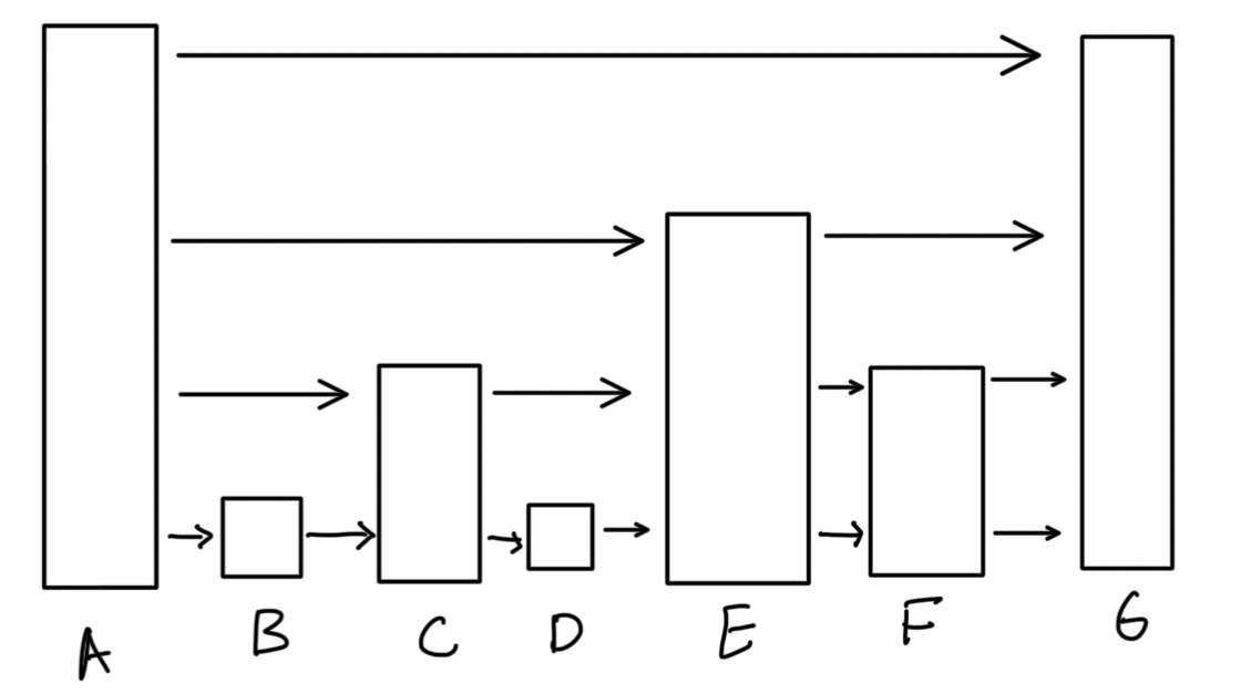
First, we assume that all the nodes are sequentially ordered. Now, imagine we want to get from node A to F. Using a normal linked list, we would only have the bottom layer; we would have to traverse B, C, D, and E. However, in the skip list, we start from the topmost layer. Following is how we can think of it algorithmically:

• We start at the topmost layer. If we take the link, we end up at G, which is too far.
• we start at the next biggest layer. If we take the link, we end up at E, which is smaller than F!. We take this link, and travel to E.
• We are now at G. We check the layer we are on again — if we take the link, we end up at G. We drop down another layer.
• We drop down another layer. We take this link and end up at F! Yay!

So we get to our target node in less than half the steps it would take a normal linked list!

So that is half of our solution. Now for the next.

Navigable Small Worlds

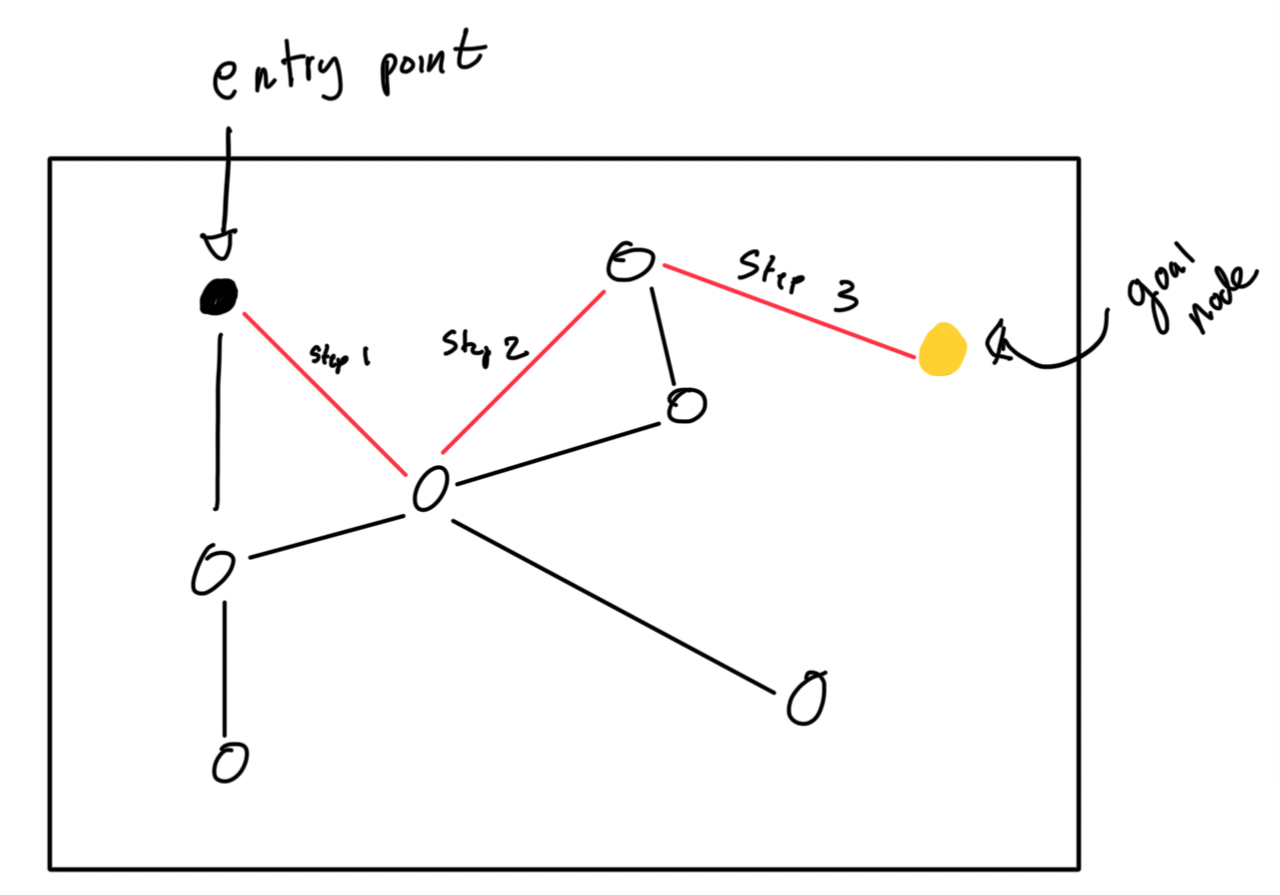
Basically, the idea is that we have a graph of nodes, where each node represents a vector stored in the database and is bidirectionally linked to some number of other nodes. We have a defined entry point E, where all searches start from. From E, we find the closest node to our query. We jump to that node. From the new node, we find the closest node to our query, and we jump to THAT node. This process is basically repeated ad-nauseam until the node we jump to is itself the closest node to the query in the whole database. Profit! I’ve illustrated this below:

Now what?

Do you see how these two can come together? This is the magic of HNSW. By combining these two ideas, we get a super-powerful data structure that is both fast and accurate. By having multiple layers of NSWs, with each layer more “specific” than the last, we are able to now search both very quickly and very accurately for the nearest neighbors of a query vector. Bingo! Below I’ve illustrated how this works.

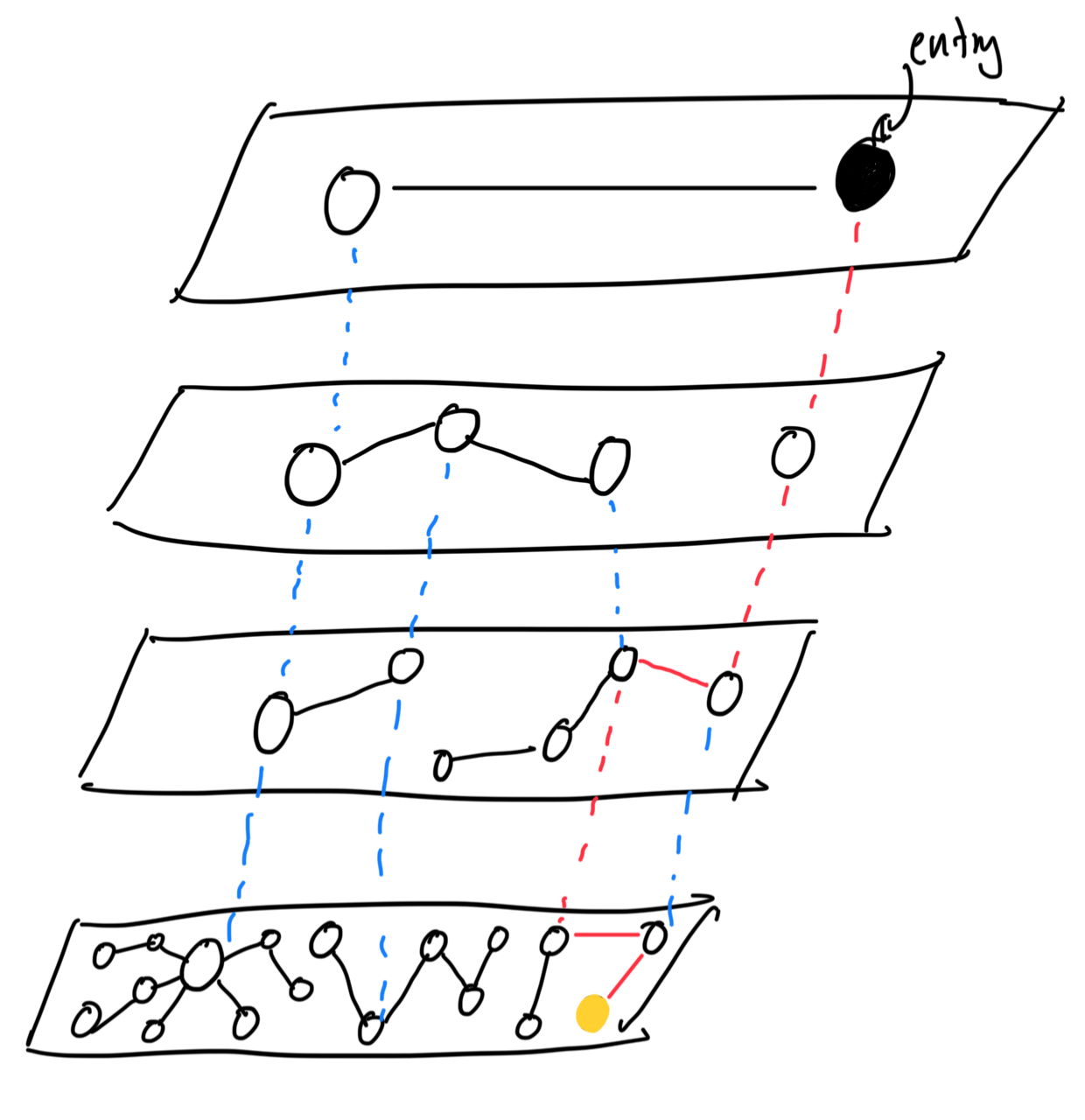
The red lines indicate the path that is taken to get to the goal node. If you notice, you’ll see that the vast majority of nodes reside on the lowest layer, and each of these nodes have a rich connection count. This fact ensures that we traverse through the top layers and find the closest node per layer as fast as possible, so that once we get to the bottom layer we just have to conduct one final search to find the nearest neighbor.

So how is this all implemented??

Here lies the fun part! Let us go through the parts step-by-step.